Uneven rent growth across rental market segments
Introduction
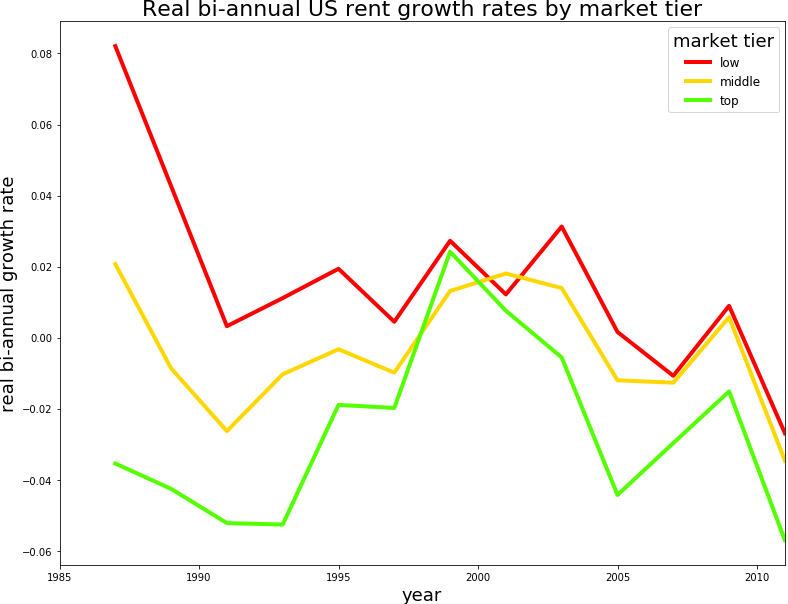
Any statement mentioning a single growth rate or unaffordability index for all rental units is bound to miss the nuance that not all segments of the rental market grow at an equal pace. As I discuss below, rents for the higher-tier rental market should grow slower than the rest of the market while rents in the low-tier market should grow the fastest. Empirical assessment of rent growth using a 1985-2011 panel of American Housing Survey data confirms this. The bi-annual growth in mid-tier real rents is 2%, -0.3% in the high-tier, and 4.1% in low-tier rents. Note, these rates are bi-annual so annual rates (in this case) are approximately half of the bi-annual rates; thus, 1% for mid-tier, -.15% for high-tier, and 2.05% for low-tier.
The above averages may conceal a lot of variation. The figure above shows that at least among the units included in this 1985-2011 AHS panel, real rent growth has not been uniform over time. Real rents among lower-tier units grew faster than the others up through the 90s but then leveled out to a slope similar to the other tiers. We also observe that rents in the highest tier seem to be most volatile.
How come we see such large differences in rent growths across the market quality segment? The set of reasons can be quite large. From differential depreciation, construction, and filtering rates to gentrification and types of facility management. In this post, I focus on the competition between the rental and ownership markets. Namely, households residing in the high-tier rental market can opt to buy property and exit the rental market while residents in low-tier housing are less likely to have such exit privileges. As a result, landlords in the high-tier compete with the ownership market while low-tier landlords only compete amongst themselves. Empirical results support this hypothesis since in times of more accessible ownership markets, growth rates in the high-tier are smaller.
Quick theory
If the upper segment of the housing rental market competes with the ownership market then rents in the upper segment will grow slower than lower tier rents. Moreover, rent growth in the upper tier should be inversely related with home-ownership accessibility. Why? Since it is generally preferable to own rather than rent, landlords renting to higher-income households will be susceptible to their renters buying into the ownership market when conditions are favourible. Consequently, landlords in this market segment compete not only against other landlords but also the ownership market. On the other hand, lower-tier landlords catering to lower-income households who are either unlikely to own or are very slow to own only compete against other landlords so they do not face this added constraint on rent-setting. As a result, higher-tier landlords have less pricing power than their lower-tier counterparts and high-end rents should grow at a slower pace than rents on the lower end of the market. Moreover, higher-tier rents should grow inversely with home-accessibility because high-tier landlords face a greater risk of renter exodus when the ownership market is easier to buy into.
Empirical Approach
I leverage the age-old repeat-sale approach to test the above hypotheses except, instead of looking at changes in home market price, I look at the change in the unit’s real rent over time. Units that start in a relatively low-tier should observe faster growth in rents than units that started in a higher tier. Assuming vertical differentiation among rental units, I define lower-tier units as any unit whose rent in the first observed year was in the bottom 25% of rents in that year. Conversely, a high-tier unit is one whose rent started in the top 25% of metro rents. Units in the middle, 25-75%, are mid-tier units. Regressing year-to-year changes in unit rents on a constant and a dummy on low and high tier units should show that relative to mid-tier units, high-tier unit rents on average grow at a slower rate and low-tier units grow at a faster rate.
Employing a similar strategy but on the sub-sample of lower and upper tier units, I also regress percent change in unit rents on home-ownership accessibility. I measure home-ownership accessibility as the interaction between mortgage interest rates and the ratio of median annual house prices to the 75th percentile of occupant renter incomes in the same year. If the price-to-income (pti) ratio is large then the gap between household incomes and home prices is large suggesting that the home-ownership market is more difficult to enter. Similarly, in case of a high interest rate, the housing market is less accessible. When both high prices and high interest rates prevail, the housing market is less accessible so the coefficient on the interaction term should be positive.
For data, I use the 1985-2011 bi-annual American Housing Survey (AHS) panel on rental units assembled by Rosenthal for his 2014 AER paper on filtering. The data are meant to be nationally representative so include units from over 147 metropolitan areas (SMSAs). To control for this, I include a SMSA fixed effect in the regressions. The repeat-sale approach typically uses change of ownership in houses to register changes in home values but since rents can change without change of occupant, I examine all bi-annual changes in rents and include a dummy for whether the unit retains its previous tenant or not. Per usual, percent change in rents is approximated by the log ratio of a unit’s rent in years t+2 and t. The price to income ratio is estimated using the home values of home owners who have lived in their dwelling for less than 10 years and the 75th percentile of renter occupant incomes. All rents have been deflated by the US average all-item CPI (though all-item less shelter is a more standard approach). I exclude units with bi-annual growth over 100%.
Results
| Dependent variables. | ||
| rent change | high-tier rent change | |
|---|---|---|
| p-values in parentheses. | ||
| Intercept | 0.020 (0.254) | -0.019 (0.597) |
| higher-tier | -0.023 (0.000) | |
| low-tier | 0.021 (0.000) | |
| r:pti | 0.035 (0.520) | |
| same HH | -0.014 (0.000) | -0.005 (0.064) |
| nObs | 145163 | 37111 |
| R^2 adj | 0.01 | 0 |
| condNum | 425 | 1743 |
Results concur with expectations outlined above. In the ‘rent change’ column of the above table, I regress bi-annual changes in real rents on a low-tier and high-tier unit dummies as defined. The intercept suggests that mid-tier market rents grew at an average 2% every two years though this estimate is not distinguishable from 0 even at the 10% level. The coefficient on high-tier units implies that real rents grew bi-annually by -.3% (or 2.3pp less than mid-tier). Low-tier unit rents grew by 4.1% every two years suggesting that rents in that segment grew fastest. This confirms the expectation that high-tier unit rents grow at a slower pace than low-tier units.
In the ‘high-tier rent change’ column, I regress rent changes among top-tier units on the price-to-income (pti) ratio interacted with the average annual mortgage interest rates (r). The positive coefficient on r:pti implies that years in which the ownership market is more inaccessible, rents grow faster suggesting competition between the ownership and high-tier rental market. Alas, the coefficient on the interacted term between the interest rate and pti is non-significant. I suspect this is the case either because I am using the national average interest rate which adds noise or because the relationship between ownership markets and high-tier rents is somewhat endogenized by the fact that cities are not closed. A more rigorous test between home-ownership access and rents would involve estimates of the demand for the city’s housing through something like Bartik Shocks or, more simply, unemployment
Discussion
Beside competition with the ownership market, what else could explain the trends? Regression to the mean can certainly be a cuplrit. Namely, as time goes on, high-tier units converge in quality to lower-quality units through deterioration and replacement so rents should also converge toward the average. This will bias the coefficient on higher-tier units downward. Conversely, low-tier units deemed no longer qualified to be occupied by either the market or bureaucrats fall out. This unit survival likely lends to an upward bias on the low-tier dummy. These effects are likely minor, however, since estimates on units that are present from the beginning (1985 & 1987) of sample are nigh identical to estimates on all units.
There are a few more caveats. Renter property prices do not remain dormant through a property’s lifetime. If the property changes hands and home prices are going up, ie pti is growing, then the rental property will also cost more and rents will rise. In the data, I observe neither change of ownership nor changes in the property’s value which may endogenize pti. Another oft-cited issue is the key assumption in all repeat-sales models: both unit and neighborhood characteristics remain constant across time. This is unlikely to be the case. Nor are the valuations of these characteristics are likely to remain constant.
Code Data and STATA
The notebook used to wrangle the data and estimate the models can be found on Github. Additionally, because I use Rosenthal data (and code) from his 2014 AER paper, Are Private Markets and Filtering a Viable Source of Low-Income Housing? Estimates from a “Repeat Income” Model, I also post python code used to change the paths in the STATA program files so that Rosenthal’s data can be recreated. As a side note, I used some old STATA 13 installation I found on my laptop to run his code but I also tried on machines with newer STATA. Using newer STATA runs into countless problems which I could not debug though, I’m guessing if you use STATA, then you’re used to such incumbrances.